A decision tree is a supervised learning technique that can be used for both classification and regression problems but is often preferred for solving classification problems. It is a tree-structured classifier, where internal nodes represent features of the dataset, branches represent decision rules, and each leaf node represents an outcome.
- A decision tree consists of two nodes: a decision node and a leaf node. Decision nodes are used to make some type of decision and have many branches. Leaf nodes, on the other hand, are the output of those decisions and do not contain any further branches.
- The decision or test is made based on the characteristics of the specified dataset.
- It is a graphical representation of all the possible solutions to a problem/decision based on the given conditions.
- It is called a decision tree because, like a tree, it starts from the root node and branches out to form a tree-like structure.
- Use the CART algorithm to build the tree. This stands for Classification and Regression Tree Algorithm.
- Decision trees simply ask a question and then split the tree into subtrees based on the answer (yes/no).
Why use decision trees?
There are many different algorithms in machine learning, so choosing the best algorithm for your particular dataset and problem is the main point to keep in mind when building a machine learning model. There are two reasons for using decision trees:
Decision trees are generally easy to understand because they mimic the human ability to think when making decisions.
Decision trees show a tree-like structure, making it easy to understand the logic behind them.
Decision Tree Terminologies
- Root Node: The root node is the starting point of the decision tree. It represents the entire dataset, which is further divided into two or more homogeneous sets.
- Leaf Nodes: Leaf nodes are the last output nodes, and the tree cannot be divided further after obtaining the leaf node.
- Partitioning: Partitioning is the process of dividing the decision node/root node into subnodes according to specified conditions.
- Branch/subtree: a tree formed by splitting a tree.
- Pruning: Pruning is the process of removing unwanted branches from a tree.
- Parent/child nodes: The root node of the tree is called the parent node, and other nodes are called child nodes.
How does the Decision Tree algorithm work?
In a decision tree, an algorithm to predict classes for a given dataset starts at the root node of the tree. The algorithm compares the value of the root attribute with the record (actual dataset) attribute and follows the branch to go to the next node based on that comparison.
At the next node, the algorithm compares the attribute value again with other subnodes and moves on. This process continues until a leaf node of the tree is reached. The algorithm given below will help you understand the entire process better.
- Step 1: Start the tree at the root node (let’s call it S), which contains the entire dataset.
- Step 2: Use Attribute Selection Measurement (ASM) to find the best features in the dataset.
- Step 3: Divide S into subgroups with the best possible values of the attribute.
- Step 4: Generate decision tree nodes with optimal features.
- Step 5: Recursively create a new decision tree using a subset of the dataset created in step 3. We continue this process until we reach the stage where we cannot classify the nodes any further and call the last nodes leaf nodes.
Example: A candidate has a job offer, and you want to decide whether to accept the offer. Therefore, to solve this problem, the decision tree starts from the root node (salary attribute as per ASM). The root node is divided into the next decision node (distance to office) and a leaf node based on the corresponding label. The next decision node is divided into a decision node (CAB function) and a leaf node. Finally, the decision node is divided into two leaf nodes: an accepted proposal and a rejected proposal. Consider the picture given below.
Attribute Selection Measures
When implementing a decision tree, the main question arises: how to select the best features for the root node and subnodes? To solve this problem, there is a method called Attribute Selection Mode (ASM). This measurement makes it easier to choose the best features for the nodes of the tree. There are two common techniques for ASM:
- information acquisition
- gini index
1. Obtaining Information:
- Information gain is a measure of the change in entropy after dividing a dataset based on an attribute.
- Calculate how much information the feature provides about the class.
- Divide the nodes and build a decision tree according to their information gain values.
- Decision tree algorithms always try to maximize the value of information gain, and the nodes/features with the highest information gain are split first. It can be calculated using the formula given below.
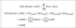
1. Information gain = entropy (S) – [(weighted average) *entropy (each feature)]
Entropy: Entropy is a metric to measure the impurity of a particular feature. Specify the randomness of the data. Entropy can be calculated as follows:.
Entropy= -P(yes) log2 P(yes)-P(no) log2 P(no)
Where,
S=total number of samples
P(yes) = probability of yes
P(No) = Probability of No
2. Gini Index:
The Gini index is a measure of impurity or purity used in building decision trees in the CART (Classification and Regression Tree) algorithm.
Properties with a lower Gini index should be preferred over those with a higher Gini index.
Create only binary partitions. The CART algorithm uses the Gini index to create a binary partition.
The Gini index can be calculated using the following formula:
Gini Index = 1- ∑jPj2
Pruning: Getting an Optimal Decision tree
Pruning is the process of removing unnecessary nodes from a tree to obtain an optimal decision tree.
Too large a tree increases the risk of overfitting, while a small tree may not capture all the important features of the dataset. Therefore, the technique of reducing the size of the training tree without reducing its accuracy is known as pruning. There are two main types of tree pruning techniques used.
Reduction in cost complexity
Error sorting is reduced.
Advantages of the Decision Tree
It is easy to understand as it follows the same process that humans follow while making decisions in the real world.
- Very useful in solving decision-related problems.
- It helps you think about all the possible outcomes of a problem.
- Requires less data cleaning than other algorithms.
Disadvantages of the Decision Tree
- Decision trees have many layers and, hence, are complex.
- There may be a problem of overfitting, which can be solved using the random forest algorithm.
- Increasing the number of class labels can increase the complexity of computing the decision tree.
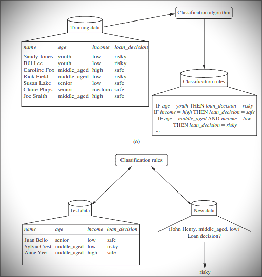
An example of creating a decision tree:
Learning phase: Training data is input into the system and analyzed by the classification algorithm. In this example, the class label attribute is “Loan Decision. The models built from this training data are represented as decision rules.
Classification: A test dataset is fed into the model to check the accuracy of the classification rules. If the model produces acceptable results, it is applied to a new dataset with unknown class variables.
Decision Tree Induction Algorithm

You should know more about decision tree:
Decision Tree Induction
Decision tree induction is a method of learning decision trees from a training set. The training set contains features and class labels. Applications of decision tree induction include astronomy, financial analysis, medical diagnostics, manufacturing, and production.
A decision tree is a flowchart tree-like structure built from training set tuples. The dataset is divided into smaller subsets and exists as nodes in a tree. A tree structure consists of a root node, internal or decision nodes, leaf nodes, and branches.
The root node is the topmost node. It represents the best features selected for classification. The internal nodes of a decision node represent tests of features, and the leaf or terminal nodes in the dataset represent classification or decision labels. The branch displays the results of the tests executed.
Some decision trees contain only binary nodes. This means exactly two branches of a node, but some decision trees are non-binary.
The image below shows a decision tree from the Titanic dataset to predict whether passengers will survive or not.

CART
CART models, or classification and regression models, are decision tree algorithms for building models. Decision tree models whose target values vary in nature are called classification models.
Discrete values are a finite or countable infinite set of values. For example, age, size, etc. Models where the target value is expressed as a continuous value, usually numerical, are called regression models. Continuous variables are floating-point variables. These two models together are called CART.
CART uses the Gini index as a classification matrix.
Decision Tree Induction for Machine Learning: ID3
In the late 1970s and early 1980s, J. Ross Quinlan was a researcher who created the decision tree algorithm for machine learning. This algorithm is known as ID3 (Iterative Dichotomyser). This algorithm was developed by E.B. Hunt, J. And the concept described by Marin is an extension of the learning system.
ID3 later became known as C4.5. ID3 and C4.5 follow a greedy top-down approach to building decision trees. The algorithm starts with a training dataset containing class labels that is divided into smaller subsets during tree construction.
- Initially, there are three parameters: attribute list, attribute selection method, and data partition. The attribute list describes the characteristics of the training set tuple.
- The feature selection method explains how to select the best features to discriminate between tuples. The methods used to select features are either information gain or the Gini index.
- The structure of the tree (binary or non-binary) is determined by how the features are selected.
- When building a decision tree, the decision tree starts as a single node representing a tuple.
- If the tuple at the root node represents different class labels, call the attribute selection method to split or divide the tuple. This step leads to the creation of branches and decision nodes.
- The partition method determines which features should be selected to partition the data tuple. Further, based on the test results, we decide which branches to develop from the node. The main purpose of the partitioning criterion is that the partitioning of each branch of the decision tree should represent the same class label.
An example of a splitting attribute is shown below:
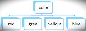
a. The portioning above is discrete-valued.
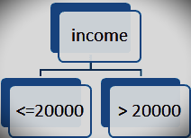
b. The portioning above is for continuous value.
Perform the above partitioning steps recursively to build a decision tree for the 7 training dataset tuples.
8. Partitioning stops only when all partitions have been created or when the remaining tuples cannot be divided further.
9. The complexity of an algorithm is denoted by n * |D|, which is represented by. * log |d|, where N is the training dataset D and |D| is the number of features.
What is greedy recursive binary splitting?
In the binary partition method, tuples are partitioned, and a cost function is calculated for each partition. The lowest cost partition is selected. The splitting method is binary, which is formed in the form of two branches. It is recursive in nature, as the same method (calculating the cost) is used to split other tuples in the dataset.
This algorithm is called greedy because it only focuses on the current node. The focus has been on reducing costs, and other points have not been taken into account.
How Do You Select Attributes for Creating a Tree?
The attribute selection criteria used to determine how to split a tuple are also known as partitioning rules. Split criteria are used to optimally split the dataset. These measures provide rankings on features to split the training tuples.
The most common way to choose features is information gain, or the Gini index.
Information Gain
This method is the main method used to create decision trees. This reduces the information required to classify tuples. This reduces the number of trials required to classify a given tuple. The feature with the highest information gain is selected.
The basic information required to classify tuples in dataset D is as follows:

Here, p is the probability that a tuple belongs to class C. Information is encoded in bits, so base-2 logarithms are used. E(s) represents the average amount of information required to find class labels in dataset D. This information gain is also called entropy.
After segmentation, the information required for accurate classification is obtained using the following formula:.
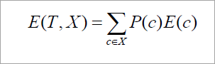
Where P (c) is the partition weight. This information represents the information needed to classify dataset D when divided by X. Information gain is the difference between the original and expected information required to classify tuples in dataset D.

The advantage is the reduction in information needed to find the value of X. The feature with the highest information gain is selected as “best.”.
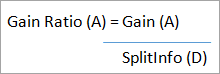
Gain Ratio
The retrieval of information may fragment parts that are not useful for classification. However, the gain ratio divides the training data set into partitions and considers the number of resulting tuples relative to the total tuples. The attribute with the highest profit percentage is used as the segmentation attribute.
Gini Index
The Gini Index is calculated for binary variables only. It measures the impurity in training tuples of dataset D, as
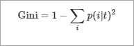
P is the probability that tuple belongs to class C. The Gini index that is calculated for binary split dataset D by attribute A is given by:
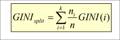
Where n is the nth partition of the dataset D.
The reduction in impurity is given by the difference between the Gini index of the original dataset D and the Gini index after partitioning by feature A.
The maximum reduction of impurities, or maximum Gini index, is chosen as the best feature for segmentation.
Overfitting In Decision Trees
Overfitting occurs when a decision tree attempts to become as perfect as possible by increasing the depth of testing, thereby reducing errors. This makes the tree too complex and causes overfitting.
Overfitting makes decision trees less predictable. Ways to avoid excessive felling of trees include pruning before and after pruning.
What is tree pruning?
Pruning is a method of removing unused branches from a decision tree. Some branches of the decision tree may represent outliers or noisy data.
Pruning is a method of reducing unnecessary branches on a tree. This reduces the complexity of the tree and aids in effective predictive analysis. It reduces overfitting by removing unimportant branches from the tree.
There are two ways of pruning the tree:
Pre-pruning: This approach stops decision tree construction early. This means that now it has been decided not to split the branch. The last node created becomes the leaf node, which potentially contains the most frequent class among the tuples.
Attribute selection measures are used to examine divided weights. Boundaries are specified to determine which partitions are considered useful. If splitting a node results in partitions below the limit, the process will stop.
Post-pruning: This method removes outer branches from a fully grown tree. Unnecessary branches are removed and replaced with leaf nodes that represent the most frequently used class labels. This technique requires more calculations than pre-pruning but is more reliable.
Pruned trees are more accurate and dense than unpruned trees, but they have the disadvantage of repeatability.
Repetition occurs when the same feature is tested multiple times on branches of the tree. Replication occurs when duplicate subtrees exist within a tree. These problems can be solved by multivariate partitioning.
The below image shows an unpruned and pruned tree.

Example of Decision Tree Algorithm
Constructing a Decision Tree
For example, consider the characteristics of a weather dataset from the past 10 days: visibility, temperature, wind, and humidity. The result will be variable, whether cricket is played or not. Create a decision tree using the ID3 algorithm.
| Day | Outlook | Temperature | Humidity | Wind | Play cricket |
| 1 | Sunny | Hot | High | Weak | No |
| 2 | Sunny | Hot | High | Strong | No |
| 3 | Overcast | Hot | High | Weak | Yes |
| 4 | Rain | Mild | High | Weak | Yes |
| 5 | Rain | Cool | Normal | Weak | Yes |
| 6 | Rain | Cool | Normal | Strong | No |
| 7 | Overcast | Cool | Normal | Strong | Yes |
| 8 | Sunny | Mild | High | Weak | No |
| 9 | Sunny | Cool | Normal | Weak | Yes |
| 10 | Rain | Mild | Normal | Weak | Yes |
| 11 | Sunny | Mild | Normal | Strong | Yes |
| 12 | Overcast | Mild | High | Strong | Yes |
| 13 | Overcast | Hot | Normal | Weak | Yes |
| 14 | Rain | Mild | High | Strong | No |
Step 1: The first step will be to create a root node.
Step 2: If all results are yes, then the leaf node “yes” will be returned; otherwise, the leaf node “no” will be returned.
Step 3: Find out the entropy of all observations and the entropy with attribute “x,” that is, E(S) and E(S, x).
Step 4: Find out the information gain and select the attribute with the highest information gain.
Step 5: Repeat the above steps until all attributes are covered.
Calculation of Entropy:
Yes No
9 5

If entropy is zero, it means that all members belong to the same class and if entropy is one then it means that half of the tuples belong to one class and one of them belong to other class. 0.94 means fair distribution.
Find the information gain attribute which gives maximum information gain.
For example, “Wind” takes two values: strong and weak; therefore, x = {Strong, Weak}.
Find out H(x), P(x) for x =weak and x = strong. H(S) is already calculated above.
Weak= 8
Strong= 8

For “weak” wind, 6 of them say “Yes” to play cricket and 2 of them say “No”. So entropy will be:

For “strong” wind, 3 said “No” to play cricket and 3 said “Yes”.
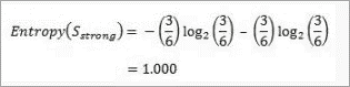
This shows perfect randomness as half items belong to one class and the remaining half belong to others.
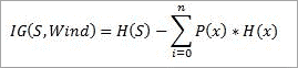
Calculate the information gain.
Similarly the information gain for other attributes is:
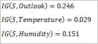
The attribute outlook has the highest information gain of 0.246, thus it is chosen as root.
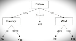
Overcast has 3 values: Sunny, Overcast and Rain. Overcast with play cricket is always “Yes”. So it ends up with a leaf node, “yes”. For the other values “Sunny” and “Rain”.
The table for Outlook as “Sunny” will be:
| Temperature | Humidity | Wind | Golf |
| Hot | High | Weak | No |
| Hot | High | Strong | No |
| Mild | High | Weak | No |
| Cool | Normal | Weak | Yes |
| Mild | Normal | Strong | Yes |
Entropy for “Outlook” and “Sunny” is:
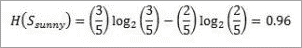
Information gain for attributes with respect to Sunny is:
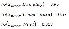
Humidity has the highest information gain and hence is selected as the next node. Similarly, entropy is calculated for rain. Wind provides the highest information gain.
The decision tree looks like this:
What is predictive modeling?
Classification models can be used to predict outcomes for unknown sets of attributes.
When a dataset with unknown class labels is input into the model, class labels are automatically assigned to the model. This method of applying probabilities to predict outcomes is called predictive modeling.
Advantages Of Decision Tree Classification
The various advantages of decision tree classification are listed below.
- Decision tree classification does not require domain knowledge and hence is suitable for knowledge discovery processes.
- The representation of data in tree format is easy and intuitive for humans to understand.
- Can handle multidimensional data.
- It is a very accurate and quick process.
Disadvantages Of Decision Tree Classification
Various disadvantages of decision tree classification are listed below.
- Decision trees can be very complex and are called overfitting trees.
- The decision tree algorithm may not be the optimal solution.
- Decision trees may return biased solutions if some class labels are dominant.
follow me : Twitter, Facebook, LinkedIn, Instagram